

What if limits are the hidden tool that turns messy change into exact answers?
They show what a function approaches as inputs get near a point, even when the function breaks or heads to infinity.
In this post I’ll explain the core idea, the epsilon–delta (formal definition), one-sided and infinite limits, key limit laws, and practical tricks like factoring and L’Hôpital.
You’ll also see clear real-world examples—motion, rates, and finance—so you can compute limits and know why they matter.
Core Meaning of Limits and How They Work

A limit tells you what value a function gets close to as the input nears a specific number, without actually arriving there. You’re not asking “what happens at this point.” You’re asking “what happens near this point.” Take (x² − 1)/(x − 1) as an example. Plug in x = 1 directly and you get 0/0, which means nothing. But factor the top to get (x − 1)(x + 1)/(x − 1), cancel the (x − 1) pieces, and you’re left with x + 1. As x gets close to 1, that simplified version gets close to 2. So the limit is 2, even though the original function never actually hits that value when x = 1.
Limits can approach from the left, the right, or both. They can also describe what happens when x shoots toward infinity or when a function itself grows without stopping.
Common limit notation:
- lim x→a f(x) = L (the limit of f(x) as x approaches a equals L)
- lim x→a⁻ f(x) (left-hand limit, approaching from smaller values)
- lim x→a⁺ f(x) (right-hand limit, approaching from larger values)
- lim x→∞ f(x) (limit as x grows toward positive infinity)
Limits matter because they let you study behavior near points where a function might break, vanish, or change fast. They’re the backbone of derivatives (measuring instantaneous rate of change) and integrals (measuring accumulated area). Without them, you can’t rigorously define what it means to zoom in on a curve or calculate the exact slope of a tangent line at one point.
Formal Limit Definitions and the Epsilon–Delta Framework

The informal “approaching” idea becomes precise through epsilon–delta. Formally, for every ε > 0 (any tolerance you pick for how close f(x) must be to L), there’s a δ > 0 (a distance around a) such that whenever 0 < |x − a| < δ, you get |f(x) − L| < ε. Translation: if you pick x values within δ units of a (but not equal to a), the function values land within ε units of L. This definition supports derivatives, continuity, and the entire calculus structure.
Epsilon–delta lets you prove limits instead of guessing. It also catches edge cases, like functions that wiggle wildly near a point or approach different values from different sides. Most intro problems don’t make you write full epsilon–delta proofs, but understanding it shows you why certain shortcuts work and others don’t. For something simple like f(x) = 2x, you can show that lim x→3 f(x) = 6 by choosing δ = ε/2, confirming that whenever |x − 3| < δ, you get |2x − 6| = 2|x − 3| < ε.
To apply epsilon–delta to a specific function:
- Start with an arbitrary ε > 0 and work backward to find δ.
- Manipulate |f(x) − L| < ε algebraically to isolate |x − a|.
- Set δ based on that, then check that your δ forces |f(x) − L| below ε.
Types of Limits and Their Behaviors
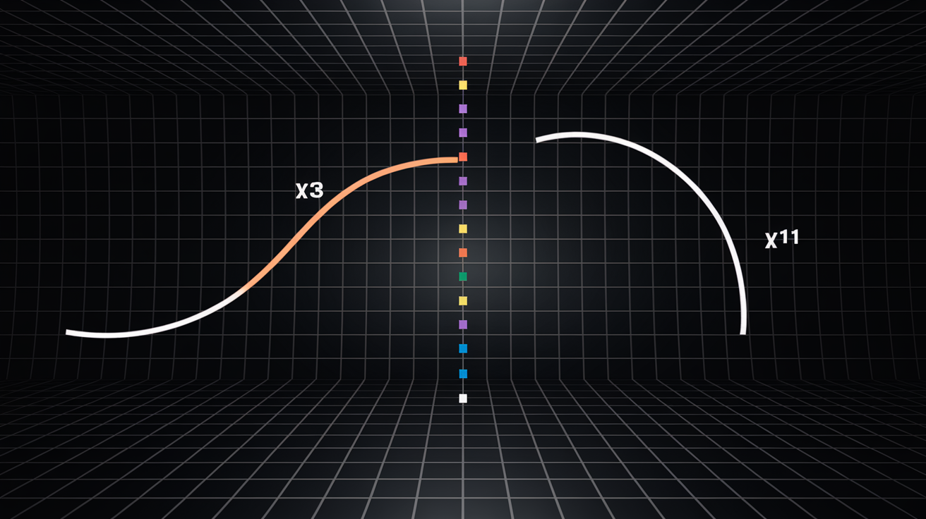
One-sided limits describe what happens when you approach from only one direction. The left-hand limit, lim x→a⁻ f(x), uses values smaller than a. The right-hand limit, lim x→a⁺ f(x), uses values larger than a. A two-sided limit exists only when both one-sided limits exist and match. Say the left-hand limit as x approaches some point equals 3.8, but the right-hand limit equals 1.3. Since those don’t agree, the ordinary (two-sided) limit doesn’t exist there. That mismatch signals a jump discontinuity, where the function breaks abruptly.
Infinite limits happen when a function grows without stopping as x nears a specific value. For instance, lim x→0 (1/x²) = +∞ means the function shoots upward as x closes in on zero. Remember, infinity isn’t a number. It’s a concept describing unbounded behavior. You can’t do arithmetic with ∞ like you do with real numbers. Expressions like “1/∞” are undefined, though we say informally they “approach zero” to describe limiting behavior.
Limits at infinity describe end behavior as x grows arbitrarily large or small. For example, lim x→∞ (1/x) = 0 because as x increases, the fraction 1/x shrinks toward zero. This type helps you understand horizontal asymptotes and long-term trends. Similarly, lim x→−∞ (1/x) = 0 shows the same shrinking when x heads toward negative infinity.
Limits of sequences extend the idea to discrete lists. If a sequence a₁, a₂, a₃, … approaches L as n increases, you write lim n→∞ aₙ = L. The sequence 1, 1/2, 1/3, 1/4, … has limit 0. Sequence limits support series convergence and bridge calculus to analysis. They also connect to topological nets and category-theory concepts like direct limits, though those show up mainly in advanced settings.
Foundational Limit Laws and Algebraic Properties

Limit laws let you split complex expressions into simpler pieces and evaluate each separately. The constant rule says lim x→a c = c (a constant’s limit is the constant itself). The sum rule states that lim x→a [f(x) + g(x)] equals lim x→a f(x) plus lim x→a g(x), if both individual limits exist. The product rule works the same way: the limit of a product is the product of the limits. The quotient rule says lim x→a [f(x)/g(x)] equals (lim f)/(lim g), but only when lim g(x) ≠ 0, since you can’t divide by zero. The power rule for polynomials gives lim x→a xⁿ = aⁿ, which means you can often substitute directly when evaluating polynomial limits.
Special trigonometric and exponential limits show up often enough to memorize. As x approaches zero, sin x / x approaches 1, which is essential for deriving the derivative of sine. Similarly, tan x / x approaches 1, and (1 − cos x)/x approaches 0. For exponential functions, (eˣ − 1)/x approaches 1 as x approaches zero, a result supporting the derivative of eˣ. Another foundational result: lim x→∞ (1 + 1/x)ˣ = e, the definition of Euler’s number (roughly 2.718281828). This limit connects exponential growth, compound interest, and continuous compounding in finance.
Key limit laws:
- Constant multiple: lim [c · f(x)] = c · lim f(x)
- Sum and difference: lim [f(x) ± g(x)] = lim f(x) ± lim g(x)
- Product: lim [f(x) · g(x)] = (lim f(x)) · (lim g(x))
- Quotient: lim [f(x)/g(x)] = (lim f(x))/(lim g(x)) when lim g(x) ≠ 0
- Power: lim xⁿ = aⁿ for positive integer n
These rules extend naturally to limits at infinity and one-sided limits. If you know lim x→∞ f(x) = 3 and lim x→∞ g(x) = 5, then lim x→∞ [f(x) + g(x)] = 8. The laws fail when individual limits don’t exist or when you hit indeterminate forms like 0/0, which need extra techniques to resolve.
Practical Techniques for Evaluating Limits

Direct substitution is simplest: plug in the value and see if you get a defined result. For example, lim x→6 (x/3) = 6/3 = 2. This works whenever the function is continuous at the point. When direct substitution gives 0/0, you’ve hit an indeterminate form, and you need to simplify before substituting. Factoring is the most common fix. For (x² − 1)/(x − 1) as x approaches 1, factor the top to (x − 1)(x + 1), cancel the (x − 1) pieces, and you’re left with x + 1, which equals 2 when x = 1.
Conjugate multiplication helps when square roots create indeterminate forms. If you have something like (√(x + h) − √x)/h, multiply top and bottom by the conjugate √(x + h) + √x to rationalize. The resulting algebra often cancels the problem term. One-sided checks are necessary when a function behaves differently on either side of a point. Compute lim x→a⁻ f(x) and lim x→a⁺ f(x) separately, then compare. If they match, the two-sided limit exists. If not, it doesn’t.
For rational functions as x approaches infinity, compare the degrees of the top and bottom. If the top’s degree is smaller, the limit is 0. If the degrees match, the limit is the ratio of the leading coefficients. If the top’s degree is larger, the limit is ±∞ depending on signs. This shortcut saves time when handling polynomials divided by polynomials at infinity.
| Technique | When It Works | Simple Example |
|---|---|---|
| Direct substitution | Function is continuous at the point | lim x→2 (3x + 1) = 7 |
| Factoring and canceling | Indeterminate form 0/0 with polynomial factors | lim x→3 (x² − 9)/(x − 3) = 6 |
| Conjugate multiplication | Square roots in numerator or denominator | lim x→0 (√(1 + x) − 1)/x = 1/2 |
| One-sided evaluation | Piecewise or absolute-value functions | lim x→0⁺ (|x|/x) = 1 |
Advanced Indeterminate Forms and L’Hôpital Applications

Indeterminate forms show up when direct substitution gives expressions like 0/0 or ∞/∞, which don’t have one well-defined value. Other indeterminate forms include 0 · ∞, ∞ − ∞, 0⁰, 1^∞, and ∞⁰. Each signals that the limit depends on how the top and bottom (or the competing terms) approach their problematic values. For example, both (x² − 4)/(x − 2) and (x − 2)/(x² − 4) produce 0/0 when x approaches 2, but the first simplifies to 4 while the second approaches 0 after cancellation. You can’t conclude anything from the indeterminate form alone. You need extra work.
L’Hôpital’s rule transforms 0/0 or ∞/∞ limits into simpler ones by replacing the original fraction with the fraction of derivatives. If lim x→a f(x)/g(x) is indeterminate 0/0 or ∞/∞, and if f'(x) and g'(x) exist near a, then lim x→a f(x)/g(x) = lim x→a f'(x)/g'(x), assuming the latter limit exists. For instance, lim x→0 (sin x)/x is 0/0, so you can differentiate top and bottom separately to get lim x→0 (cos x)/1 = 1. This matches the known special limit for sin x / x and confirms the rule’s usefulness.
To apply L’Hôpital’s rule:
- Verify that direct substitution gives 0/0 or ∞/∞.
- Differentiate the top and the bottom separately (don’t use the quotient rule).
- Evaluate the new limit. If it’s still indeterminate, apply L’Hôpital again until you reach a determinate form or conclude the limit doesn’t exist.
Continuity, Discontinuities, and How Limits Detect Breaks

A function is continuous at a point if the limit as x approaches that point equals the function’s actual value there. Formally, f is continuous at a when lim x→a f(x) = f(a). When this fails, you’ve got a discontinuity. Removable discontinuities happen when the limit exists but doesn’t match the function value (or the function isn’t defined at all). The algebraic cancellation example (x² − 1)/(x − 1) shows this: the function is undefined at x = 1, but the limit equals 2. You can “remove” the discontinuity by redefining the function to equal 2 at x = 1, making it continuous.
Jump discontinuities happen when left-hand and right-hand limits exist but don’t agree. The example where the left-hand limit equals 3.8 and the right-hand limit equals 1.3 shows a clear jump: the function value hops from one level to another without passing through in-between values. No redefinition can fix a jump, since the function genuinely behaves differently on either side. Step functions and piecewise-defined functions often show jumps at their transition points.
Essential (or infinite) discontinuities appear when at least one one-sided limit fails to exist or equals ±∞. For example, lim x→0 (1/x²) = +∞ means the function shoots upward without bound as x approaches zero. You can’t assign a finite value at zero to make the function continuous, and the behavior is fundamentally different from a removable or jump discontinuity. Essential discontinuities signal vertical asymptotes or oscillatory behavior that prevents any finite limit from existing.
Limits in Multivariable and Applied Contexts
In multivariable calculus, limits extend to functions of two or more variables. For a function f(x, y), the limit as (x, y) approaches (a, b) is written lim (x,y)→(a,b) f(x, y) = L. The formal definition mirrors the single-variable version: for every ε > 0, there’s Δ > 0 such that whenever 0 < √[(x − a)² + (y − b)²] < Δ, you get |f(x, y) − L| < ε. The key difference is that (x, y) can approach (a, b) along infinitely many paths (not just from left or right), so you must verify that f(x, y) approaches the same value regardless of the path taken.
Path dependence is a common pitfall. If f(x, y) approaches different values along different paths (say, along the x-axis versus the line y = x), the limit doesn’t exist. Iterated limits (where you take the limit in x first, then in y, or vice versa) don’t always match the true two-variable limit, even when both iterated limits exist. This subtlety makes multivariable limits trickier to evaluate and often requires switching to polar coordinates or applying squeeze-theorem arguments.
Limits show up throughout physics and engineering. Notable real-world limits:
- The speed of light (roughly 299,792,458 m/s) acts as an upper limit for the speed of any object with mass, a cornerstone of special relativity.
- Absolute zero (0 Kelvin or −273.15°C) represents the lower limit of temperature, where molecular motion theoretically stops.
- Material strength thresholds define the limit of stress a structure can handle before yielding or breaking, guiding safe design loads in civil and mechanical engineering.
- Load capacity limits in electrical circuits prevent overheating and failure, keeping components within safe current and voltage ranges.
These applied limits translate mathematical abstraction into concrete constraints, helping engineers predict failure points, optimize performance, and design systems that stay safe and efficient under varying conditions.
Common Limit Mistakes and How to Fix Them

One frequent error is treating indeterminate forms like 0/0 as if direct substitution alone resolves them. When you plug in a value and get 0/0, you haven’t found the limit. You’ve only confirmed that more work is needed. Always factor, simplify, or apply L’Hôpital’s rule before concluding anything. Another mistake is assuming that a limit equals the function value without checking continuity. A function can be undefined or discontinuous at a point even when the limit exists, so verify that lim x→a f(x) actually matches f(a) before claiming continuity.
Mismatched one-sided limits trip people up when working with piecewise functions or absolute values. If lim x→a⁻ f(x) ≠ lim x→a⁺ f(x), the two-sided limit doesn’t exist, no matter what the function value at a might be. Always compute both one-sided limits separately when you suspect a break or jump. Ignoring domain restrictions is another pitfall: forgetting that the denominator can’t be zero, or that a square root requires non-negative inputs, leads to nonsense answers. Check the domain before applying limit laws, and note any points where the function isn’t defined.
Common mistakes and quick fixes:
- Assuming 0/0 = 0 or undefined: Factor and cancel, or use L’Hôpital’s rule.
- Ignoring one-sided limits in piecewise functions: Compute left and right limits separately, then compare.
- Dividing by zero without catching it: Verify the denominator’s limit isn’t zero before applying the quotient rule.
- Confusing limits at infinity with limits of infinity: Limits at infinity describe end behavior. Limits of infinity mean unbounded growth.
- Forgetting that ∞ isn’t a number: Never write expressions like “∞ − ∞ = 0” without careful justification. Use proper limit notation and algebraic techniques instead.
Final Words
We started by showing limits as “approaching” with the (x^2−1)/(x−1) → 2 example, then unpacked the epsilon-delta idea and common notations. We also mapped one-sided, infinite, and sequence limits plus the main algebraic laws.
Next, you got practical tools: substitution, factoring, L’Hôpital, checks for continuity, multivariable path issues, and common mistakes to avoid. Try a few short problems—limits get easier fast, and you’ll build real confidence quickly.
FAQ
Q: What do you mean by limit?
A: A limit means the value a function’s output approaches as the input gets close to a point, for example (x^2−1)/(x−1) approaches 2 near x = 1.
Q: What are the three types of limits?
A: The three common types of limits are two-sided limits, one-sided limits (left or right), and limits at infinity; each describes different approach behavior of a function.
Q: What is another name for limits?
A: Another name for limits is convergence, meaning the function’s values converge to a number; mathematicians also use terms like limit point or accumulation point in some contexts.
Q: What are the 7 rules of limits?
A: The seven common limit rules are the constant rule, identity rule, sum rule, difference rule, scalar multiple rule, product rule, and quotient rule, which let you simplify limit calculations.
